Recently, I had the pleasure of presenting original research and maps about early modern death at the 2024 American Historical Association in San Francisco. I showcased maps between 1656 and 1680 based on general bill data. That span of years offered interesting data to showcase, including the major plague outbreak in London in 1665 and the Great Fire of London a year later in 1666. But how did I actually map these years?

This blog post will not be an analysis of that data and those maps I made, but a way to show you how I accomplished what I set out, written in as plain of text as possible. I went from mapping stranger to novice, and I hope my work can help you make that jump.

Step 1: Putting Your Data-Ducks in a Row

Step one was to establish a data set to map. For me, it was easy enough. I was already working with the 1656-1680 general bills for some research I did into why these years had more deaths than christenings every year. That does not mean step 1 was complete, though. I needed to finish transcribing the set, which took some time. I can do a typical weekly bill in around 7-10 minutes, but general bills are different from weekly bills. The parishes moved much more on the document, and many disappeared entirely for a few years after the Great Fire. Therefore, I had to be diligent to ensure that the parishes were actually missing from the bill, not that I was just overlooking them. Once I had the full set transcribed and exported, my job was still not done. QGIS (the free mapping software I used) cannot read this document and map it:

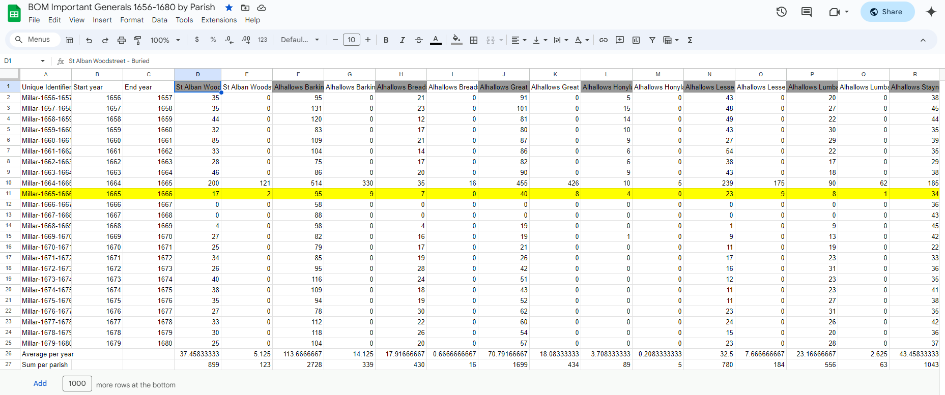
There are a few mini steps I need to do to make this usable by QGIS. First, I need to decide which information is important from this long document of stats (you only see the beginnings of the A-parishes, there are MANY more parishes that require scrolling to). I decided I wanted yearly maps, with parish names, and burials, but not cumulative burials for groupings of parishes. The best way I found for getting the data I wanted without destroying this original document showing me numbers for all categories was…transcribing all of it over again, for the most part. To re-transcribe this data, I would hide all columns other than burials and the year, and created a whole new spreadsheet with one year and all deaths per parish, but I had to do some fiddly work with the parish names. For QGIS to read my data and the shapefiles together, I would need to have at least one column on each with the exact same entries for a clean join. So I went into a random test map using our shapefiles and found a category to copy. Here are the steps I took:

• Download shapefiles from our Github.
• Open QGIS (I used QGIS 3.32 Lima for reference)
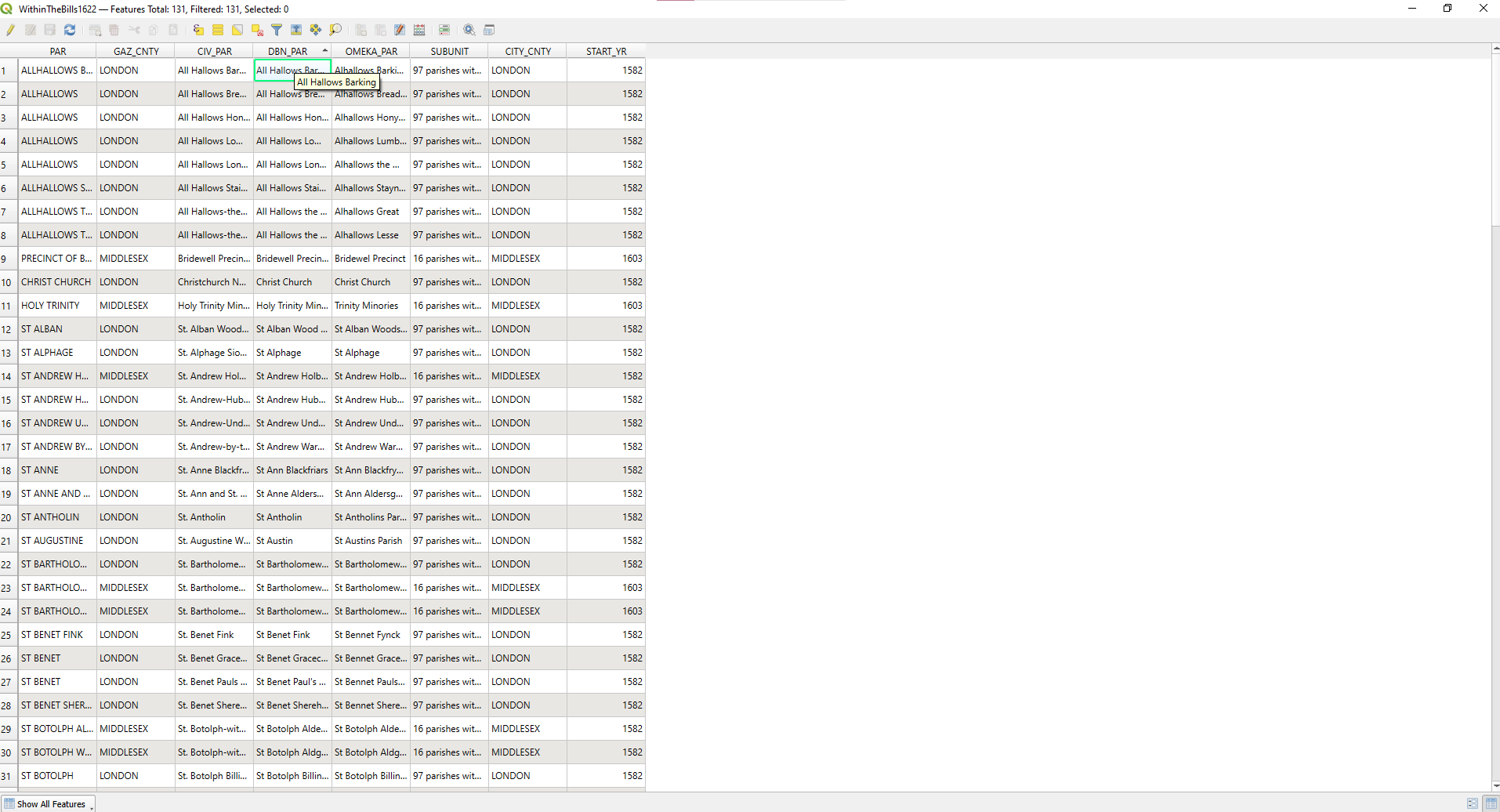
• Open the shapefile I plan on using: Layer > Add Vector Layer > Add shapefiles (.shp extension) that I downloaded from Github (bom-main> bom-data> parish-shapefiles>pick the year you want (I chose 1622 through 1671 since they were the next earliest sets for my data, but only pick one at a time per map> “WithinTheBills1622.shp”> Open>Add>Close Vector Window.
• Check Attribute Table: Go to the Layers panel on the side > Right-click on “WithinTheBills1622” > Open Attribute Table.
• Choose joinable column. You’ll likely want to differentiate between parishes if you’re mapping, so I would choose one of the parish name columns. There are 3 different parish name columns on these shapefiles. I chose the DNB_PAR column, since I knew that DBN (Database Name) values were unique.

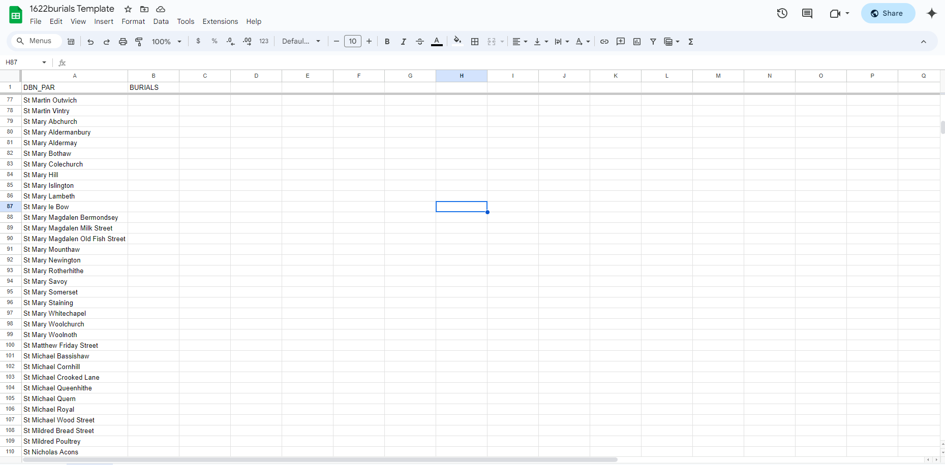
• Open an empty spreadsheet. I’d recommend naming it something like “1622 Mapping Template,” but that’s up to you and how organized you are. Then I made two columns: “DBN_PAR” (just like it’s written in the attribute table. It needs to be identical) and “BURIALS”. Then I copied every DBN_PAR item in the column to the matching spreadsheet column, making sure I had the right amount of rows compared to the attribute table. (I used ctrl-c and ctrl-v to make sure the names were identical to their original names. It doesn’t matter if they’re in the right order, but it is important that the names are the exact same.) You should have something like this:

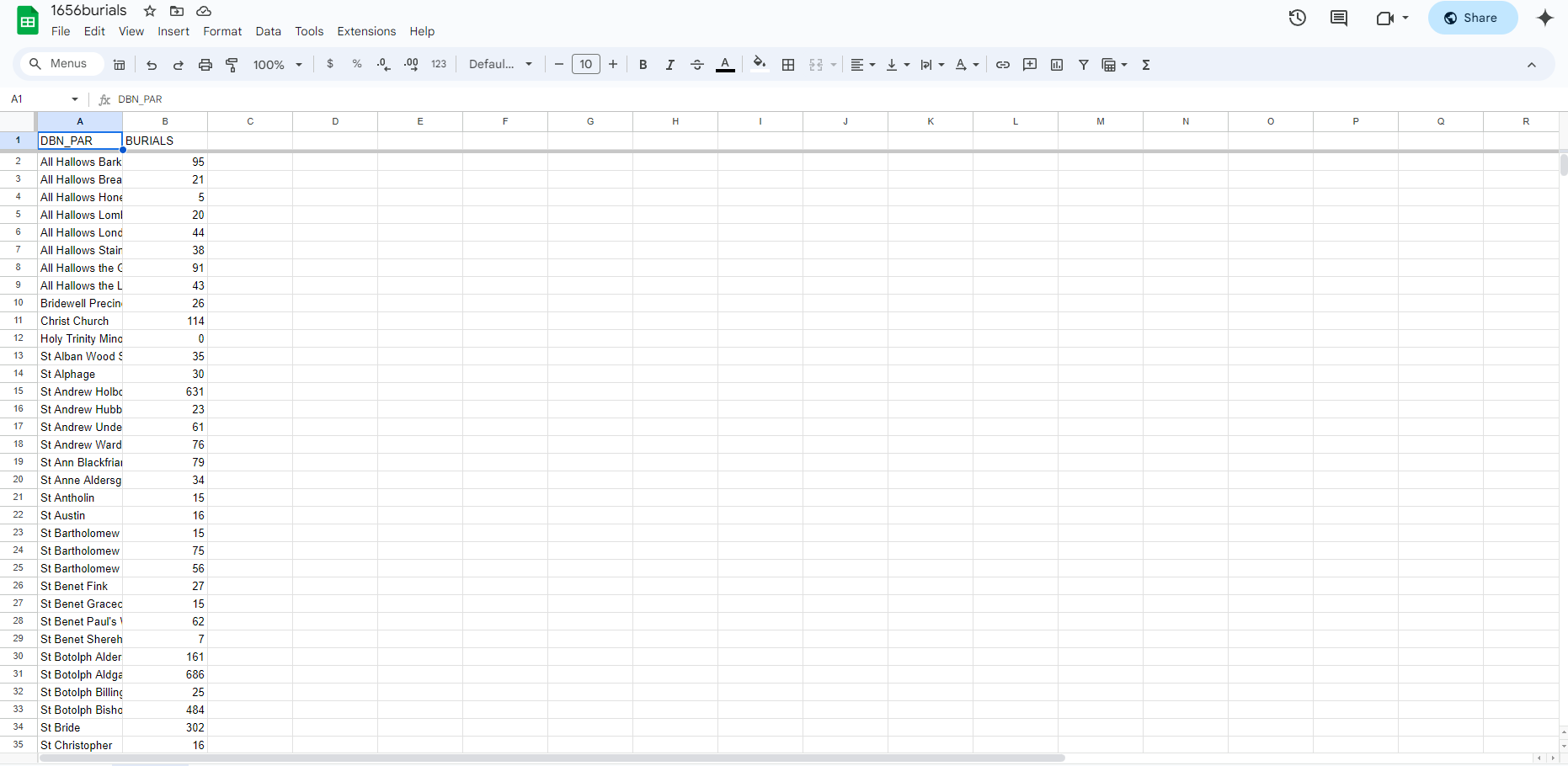
• Now make a copy of that template, name it for the first year you intend to map, and individually add the burial counts for each parish. This will take a while (especially if you plan on mapping twenty-four years like I did), so grab a drink and put on a nice playlist to listen to and get to work.
• (If you’re familiar with Spongebob, you can imagine one of those time-change cards that reads “Many Spreadsheets Later”). Then you should have at least one document that looks like this for each year you intend to map:

• Now you take that new spreadsheet you just made > file > Download > Comma Separated Values (.csv). Once you’ve downloaded it, put it somewhere easy to find (I personally made a custom folder on my desktop for mapping stuff for this project). You’ll also want to make sure it’s named something unique enough that you know what it is, but simple enough to copy by hand. My file named itself 1656burials -Sheet1.csv which isn’t terrible, but I decided to shorten it to “1656burials.csv” to make it even simpler, because the next step is weird.
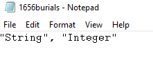
• Make a matching .csvt file. (Note: I’m not sure how necessary this step actually is, but I wasn’t able to figure out how to get it to work before I knew how to do it, so it became one of the many steps involved once I got the map to work for the first time). In the same folder that you’re storing your .csvfile, right-click in the folder > New >Text Document> Open “New Text Document”> Type: “String”, “Integer” > Save As1656burials.csvt.

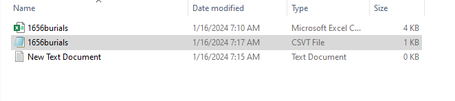
Note the name is the same as your spreadsheet, except the extension ends with a t. If it worked for you like it did for me, your folder should look like this:

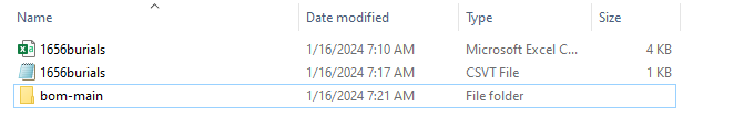
• You can delete the “New Text Document” document now, it was only needed to make a .csvt file. While we’re at it, you might want to drag the entire bom-main file you downloaded from GitHub to this folder, just to make it easier for you (it may require you to re-add the vector layer with the shapefiles in QGIS if you do this, since QGIS might forget where you put the shapefiles if you move it).

• Believe it or not, but you’re finally at the step where you can attempt to map your data!

Step 2: Joining your CSV to your SHP

Once you have all your data ducks in a row, every data set has a .csv and .csvt file. Now we can actually begin importing the data:

• Open QGIS
• Either begin with the test map that currently contains the .shp from when you tested them to get the DBN_PAR column, or create a new map, adding the .shp like we did in that first testing step. Now that you’ve got QGIS showing the .shp, you should see a map of London showing tons of parishes and all in the same color. To make the map reflect colors that mean something to us, we need to add our dataset. (Note: QGIS randomizes what color it makes the .shp when it displays for the first time. Don’t be surprised if your .shp is green, yellow, or any other color. The current color doesn’t matter in the long-run, since we’ll be changing it later.)

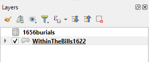
• To add our premade dataset: Layer > Add Layer > Add Vector Layer > Vector Database >Find your .csv file and open it > Add and close out of Vector interface. (If this sounds familiar, it is! It’s exactly how you add the .shp!)
• Now you should see that there are two items in the “layers” interface. For me they’re named 1656burials (with an icon that looks like a spreadsheet) and WithinTheBills1622 (with an icon that looks like a bean). These are your .csv and .shp files respectively.

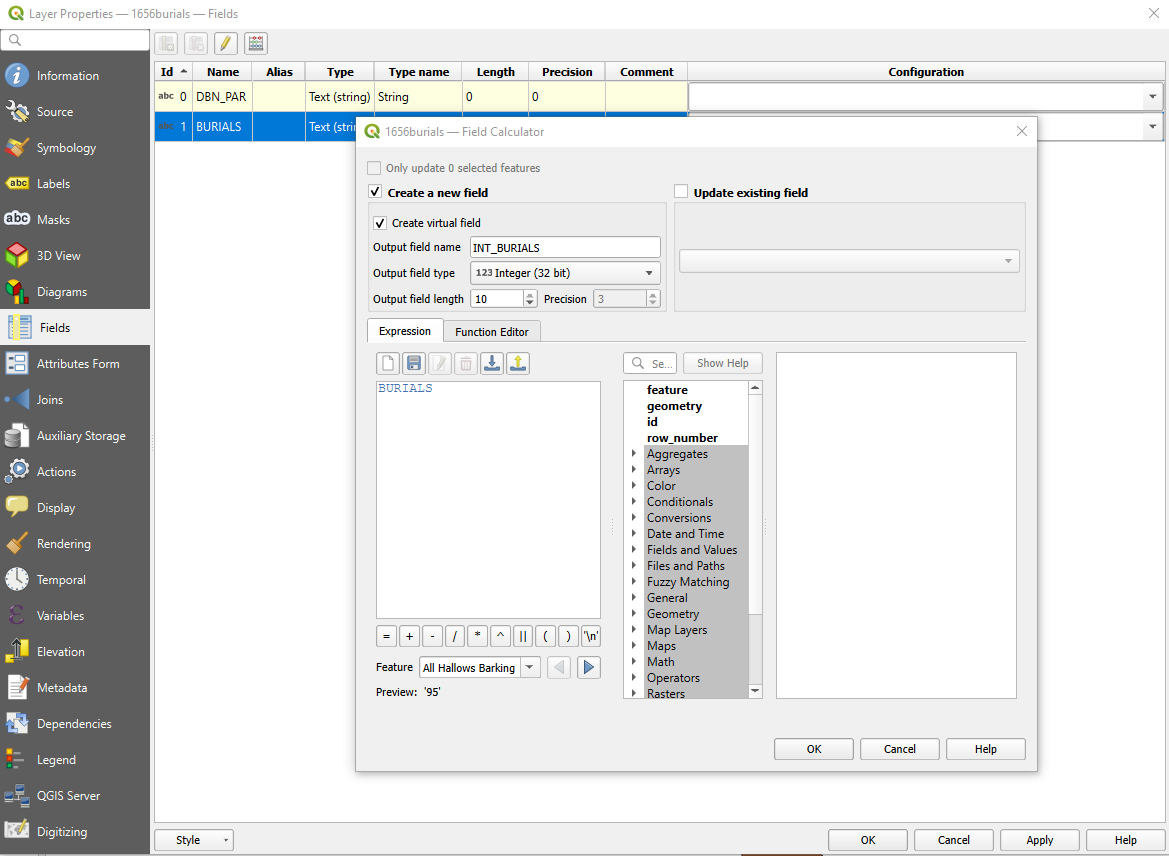
• You’ll want to right-click on the layer with the spreadsheet icon > Properties > Fields > Click on the Abacus-icon on the top > click the box for Create a New Field > click the box for Create a Virtual Field > type in output field name “INT_BURIALS” > Make sure the output field type is Integer > Type in expression box “BURIALS” > On the bottom left of this window, it should show a preview of a number that represents the burials for a feature (parish). > Click OK > Click Apply > Close Window. (Here’s what the window should look like before you commit changes). Now when you check the attribute table for the layer with the spreadsheet icon, you should see three columns: DBN_PAR, BURIALS, and INT_BURIALS. By doing this, you guarantee QGIS can read your burial numbers as numbers (which it can possibly do using the CSVT files, but it’s not always successful).

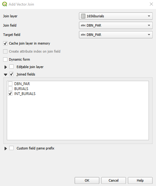
• Now that you’ve got your integers, you’ll want to join them to the .shp, which is the layer with the icon that looks like a bean. (It’s also the layer that has a box colored the same way as your map). Right click on that shapefile layer and click on properties > joins > click on the plus button on the bottom left > join layer equals your csv file name > Join field is DBN_PAR > Target field is DBN_PAR > click on the box for joined fields > click on the box for INT_BURIALS > OK > Apply > Close out of properties window.

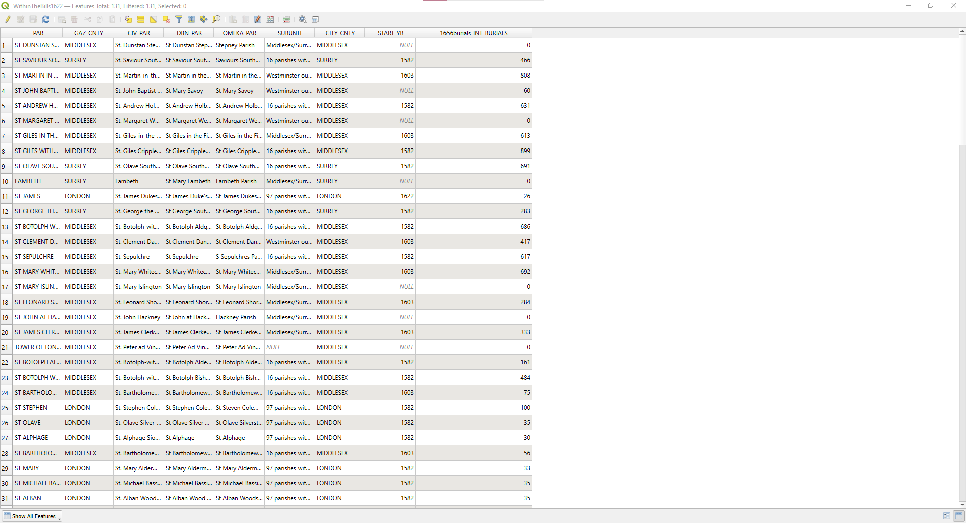
• You might think you’ve done something wrong when you close out of this window, because your map won’t look any different. But you need to check your attribute table for your shapefile and check that the INT_BURIALS column shows up (Note: It will probably have a name that combines what document it was originally from with what the column name is supposed to be, ex. 1656burials_INT_BURIALS, that’s fine).

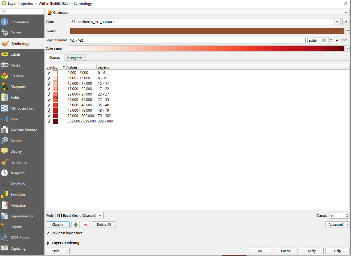
Step 3: Making the Map Actually Say Something

Now that all our shapefile and data are joined, we want the map to visually show us the data in a meaningful and readable way. I’m going to show you how I changed the symbology to reflect burials, so that every 10% of burials got darker in color. Keep in mind that you can show this data in tons of different ways. Don’t be afraid to try different modes to make the data appear in different ways.

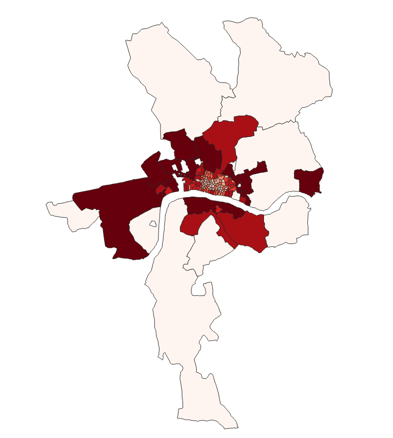
• Right click on your .shp and go to properties again, but this time we’re adding colors. Right click on .shp layer > Properties > Symbology > Change Single Fill to Graduated > Change Value to your INT_BURIALS column > Change Color ramp to one that you like. I prefer Reds > Double check your mode is Equal Quantile > Change the Class number to the amount of colors you’ll want. I like 10 so that each color represents 10% of deaths > Click Classify > Click Apply > Close Window.

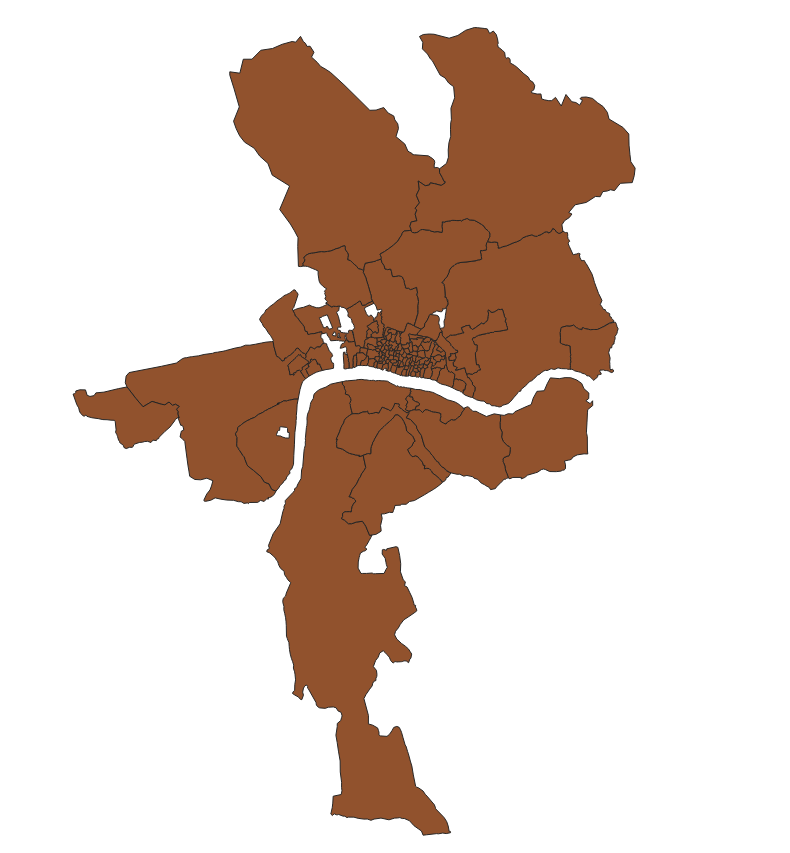
• Now when you close the window, you should see a map colored to reflect your data! Since I chose to map 1656, this means my map has a pale pink color for almost all outer parishes, since they didn’t report that early. If you choose a later year, you’ll likely have an opposite coloration, where the inner parishes are the lightest color and the outer are the darkest.

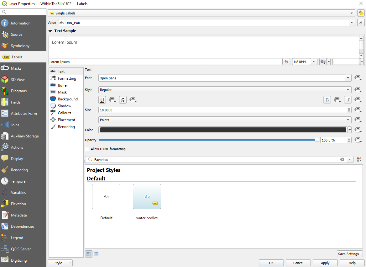
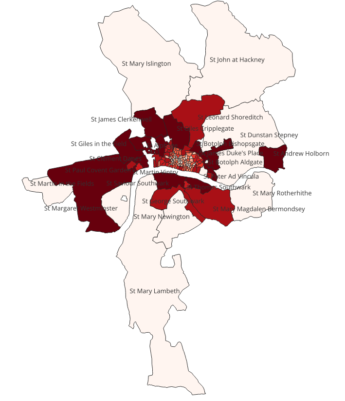
• While I don’t like leaving labels on, you could optionally also right click your shapefile layer > properties > labels > change no labels to single labels > set your value to DBN_PAR > apply > close window, to see the names of all parishes.

• Now if you only need or want the one map, you’re golden, but if you want to make a bunch of maps, Godspeed: just keep doing these same exact steps over and over again until you’ve got all your maps made.

Conclusion

These are the steps I took to create my maps of Geographical Patterns of Death in the bills from 1656 until 1680. Feel free to tweak the methods to fit your own projects. I hope this guide helps you start using our data sets and shape files to create interesting historical and statistical maps and visualizations.